5.1 Introduction

Moving averages are extremely popular with market technicians and for good reason. Moving averages smooth out the price action and make it easier to spot the underlying trends. Precise trend signals can be obtained from the interaction between a price and an average or between two or more averages themselves.

It sums up the data points of financial security over a specific time period and divides the total by the number of data points to arrive at an average. It is called a “moving” average because it is continually recalculated based on the latest price data.

The moving average is constructed by averaging several days’ closing prices, however, it tends to lag behind the price action. The shorter the average (meaning the fewer days used in its calculation), the more sensitive it is to price changes and the closer it trails the price action. A longer average (with more days included in its calculation) tracks the price action from a greater distance and is less responsive to trend changes. The moving average is easily quantified and lends itself especially well to historical testing.

5.2 Popular Moving Averages

In stock market analysis, the most popular moving average lengths are 50 and 200 days. [On weekly charts, those daily values are converted into 10 and 40-week averages.] During an uptrend, prices should stay above the 50-day average. Minor pullbacks often bounce off that average, which acts as a support level. A decisive close beneath the 50-day average is usually one of the first signs that a stock is entering a more severe correction. In many cases, the breaking of the 50-day average signals a further decline down to the 200-day average.

If a market is in a normal bull market correction, it should find new support around its 200-day average. [For short-term trading purposes, traders will employ a 20-day average to spot short-term trend changes].

5.3 Usage of Moving Averages

Securities prices, market indexes, and mutual fund prices vacillate up and down from day to day, week to week and month to month. Because of this it often becomes difficult to discern which way the prices are actually moving. A moving average is therefore used to smooth the data so that the trend can be easily detected. A rising moving-average line indicates that prices are trending up, while a declining line indicates the opposite. A flat line indicates a market stuck in a trading range and can’t seem to make up its mind which way it is going.

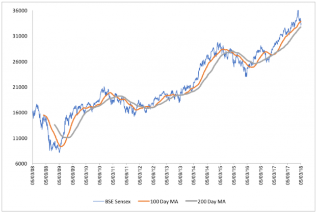
The following chart is a ten-year chart of the Sensex with a 200 DMA. The moving average is the solid line shown on the chart

You can create a moving average of any length (e.g., 10-day, 20- day, 50-day, 200-day) and for any time period (days, weeks, months) depending upon what you are trying to achieve: for example, for trading the market over short time frames a short time-frame chart would be used with a short moving average. On the other hand, investing for the long term, a long-term chart would be used with longer-term moving averages.

Many traders and investors use the moving average to help find entry and exit points. Some even use the 100 or the 200 DMA as signals to buy and sell. Meaning, the moving average is used to find points to exit the market or enter the market.

5.4 Types of Moving Averages

1. SIMPLE MOVING AVERAGE:

The SMA Is the simplest moving average that is obtained by adding the most recent data points set and then dividing the total by the number of time periods. The SMA indicator is used for traders to generate signals of when to enter or exit the stock.

An SMA is a lagging indicator as it is based on the past price data for a given period that can be computed for different types of prices such as high, low, open, and close. Traders use this indicator for determining buy, sell signals for securities and also helps to identify support and resistance zones.

Consider a situation where you want to calculate the average closing price of Britannia Limited for the latest 5 days. The data is as follows:

Hence the average closing price of Britannia over the last 5 trading sessions is Rs.3616.8.

Moving forward, the next day, i.e. 24th Jan (22^nd  and 23^nd were Saturday and Sunday respectively) we have a new data point. This implies now the ‘new’ latest 5 days would be 18^th, 19^th, 20^th, 21^st and 24th. We will drop the data point belonging to the 18^th as our objective is to calculate the latest 5-day average.

=18069/5= Rs.3613

Hence the average closing price of Britannia over the last 5 trading sessions is Rs.3613

As you can see, we have included the latest data (24^th Jan) and discarded the oldest data (17^th Jan) to calculate the 5-day average.  On 25^th, we would include 25^th data and exclude 18^th data, on 27^h, we would include 27^th data point but eliminate 20th data, so on.

We are essentially moving to the latest data point and discarding the oldest to calculate the latest 5-day average. Hence the name “moving” average!

In the above example, the calculation of the moving average is based on the closing prices.  Sometimes, moving averages are also calculated using other parameters such as high, low, and open. However, the closing prices are used mostly by the traders and investors as it reflects the price at which the market finally settles down.

Moving averages can be calculated for any time frame, from minutes, hours to years.  Any time frame can be selected from the charting software-based of your requirements.

1.       The exponential moving average

Look at this data:

When one calculates the average across these numbers, there is an unstated assumption. We are essentially giving each data point equal importance. We are assuming that the data point on 18^th Jan is as important as the data point on 24th Jan. However, when it comes to markets, this may not always be true

Remember the basic assumption of technical analysis – markets discount everything. This means the latest price you see (on 24^th Jan) discounts all the known and unknown information. This also implies the price on 24^th is more sacred than the price on 18^th or 20^th.

One would like to assign weightage to data points based on the ‘newness’ of the data. Therefore the data point on 24^th Jan gets the highest weightage, 21^st Jan gets the next highest weightage, 20^th Jan gets the 3^rd highest, and so on.

By doing so, we essentially scaled the data points according to its newness – the latest data point gets the maximum attention, and the oldest data point gets the least attention.

The average calculated on this scaled set of numbers gives us the Exponential Moving Average (EMA).

We have skipped the EMA calculation part, simply because most of the technical analysis software lets us drag and drop the EMA on prices. Hence lets understand the usage of the same rather than the calculation.

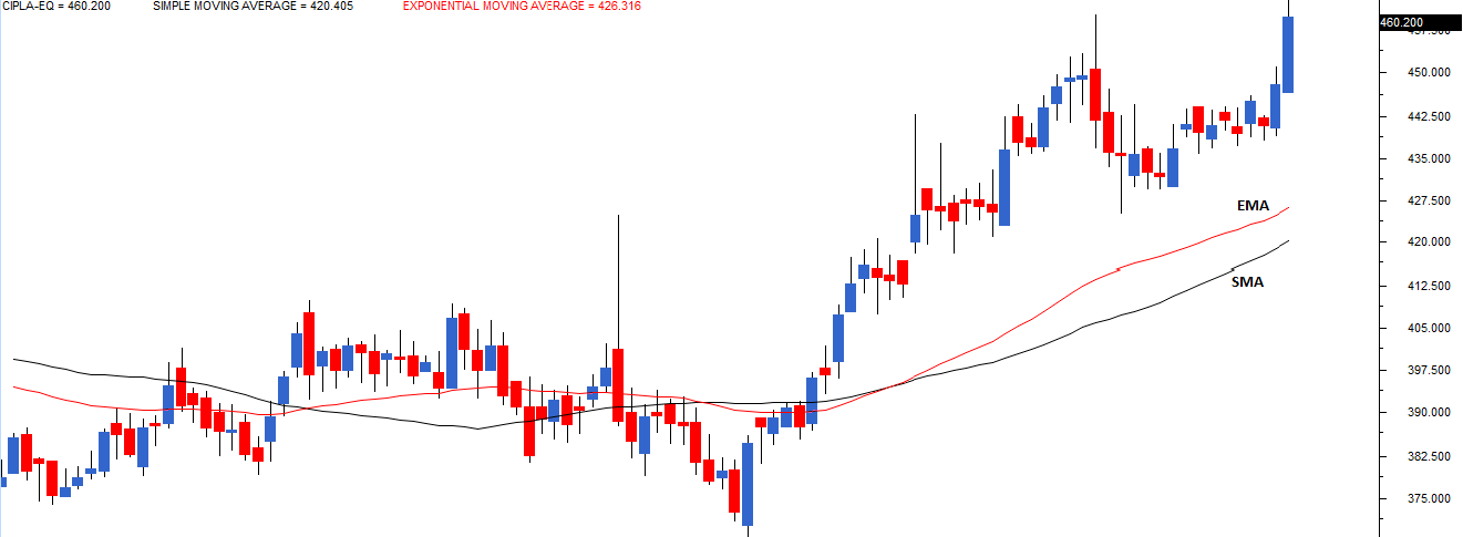
Here is a chart of Cipla Ltd. We have plotted a 50 day SMA (black) and a 50 day EMA (red) on Cipla’s closing prices. Though both SMA and EMA are for a 50 day period, you can notice that the EMA is more reactive to the prices and sticks closer to the price.

EMA is quicker to react to the current market price because EMA gives more importance to the most recent data points. This helps the trader to take quicker trading decisions. Hence, for this reason, traders prefer the use of the EMA over the SMA.

5.5 Real Life Application of Moving Averages

The moving average can be used to identify buying and selling opportunities with its own merit. When the stock price trades above its average price, it means the traders are willing to buy the stock at a price higher than its average price. This means the traders are optimistic about the stock price going higher. Therefore one should look at buying opportunities.

Likewise, when the stock price trades below its average price, it means the traders are willing to sell the stock at a price lesser than its average price. This means the traders are pessimistic about the stock price movement. Therefore one should look at selling opportunities.

We will now try and define one such trading strategy based on a 50-day exponential moving average. Lets define the moving average trading strategy with the following rules:

Rule 1) Buy (go long) when the current market price turns greater than the 50 days EMA. Once you go long, you should stay invested till the necessary sell condition is satisfied.

Rule 2) Exit the long position (square off) when the current market price turns lesser than the 50 days EMA.

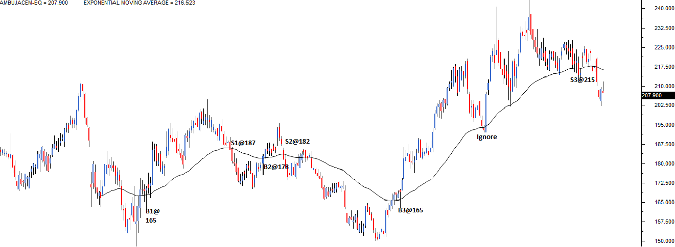
Here is a chart that shows the application of the trading system on Ambuja cement. The black line on the price chart is the 50-day exponential moving average.

Starting from left, the first opportunity to buy originated at 165, highlighted on the charts as B1@165. Notice, at point B1, the stock price moved to a point higher than its 50 days EMA. Hence as per the trading system rule, we initiate a fresh long position.

We stay invested by the trading system till we get an exit signal, which we eventually got at 187, marked as S1@187. This trade generated a profit of Rs.22 per share.

The next signal to go long came at B2@178, followed by a signal to square off at S2@182. This trade was not as impressive as it resulted in a profit of just Rs.4. However, the last trade, B3@165, and S3@215 were quite impressive, resulting in a profit of Rs.50.

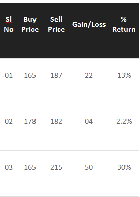
Here is a quick summary of these trades based on the trading system fared:

From the above table, it is obvious that the first and last trades were profitable, but the 2^nd trade was not so profitable. If you inspect why this happened, it is evident that the stock was trending during the 1^st and the 3^rd trade, but during the 2^nd trade, the stock moved sideways.

This leads us to a significant conclusion about the moving averages. Moving averages works brilliantly when there is a trend and fails to perform when the stock moves sideways. This basically means the ‘Moving average’ in its simplest form is a trend following system.

5.6 Moving Average Crossover System

As its evident now the problem with the plain vanilla moving average system is that it generates far too many trading signals in a sideways market. A moving average crossover system is an improvisation over the plain vanilla moving average system. It helps the trader to take fewer trades in a sideways market.

Instead of the usual single moving average in a MA crossover system, the trader combines two moving averages. This is usually referred to as ‘smoothing’.

A typical example of this would be to combine a 50 day EMA, with a 100 day EMA. The shorter moving average (50 days in this case) is also referred to as the faster-moving average. The longer moving average (100 days moving average) is referred to as the slower moving average.

The shorter moving average takes a lesser number of data points to calculate the average, and hence it tends to stick closer to the current market price and therefore reacts more quickly. A longer moving average takes more data points to calculate the average, and hence it tends to stay away from the current market price. Hence the reactions are slower.

Traders have modified the plain vanilla MA system with the crossover system to smoothen out the entry and exit points. The trader gets far fewer signals in the process, but the chances of the trade being profitable are quite high.

The entry and exit rules for the crossover system is as stated below:

Rule 1) – Buy (fresh long) when the short term moving averages turns greater than the long term moving average. Stay in the trade as long as this condition is satisfied

Rule 2) – Exit the long position (square off) when the short term moving average turns lesser than the longer-term moving average